Deriving the Black-Scholes Equation with the truncated LogNormal

12:39 AM, October 27, 2024

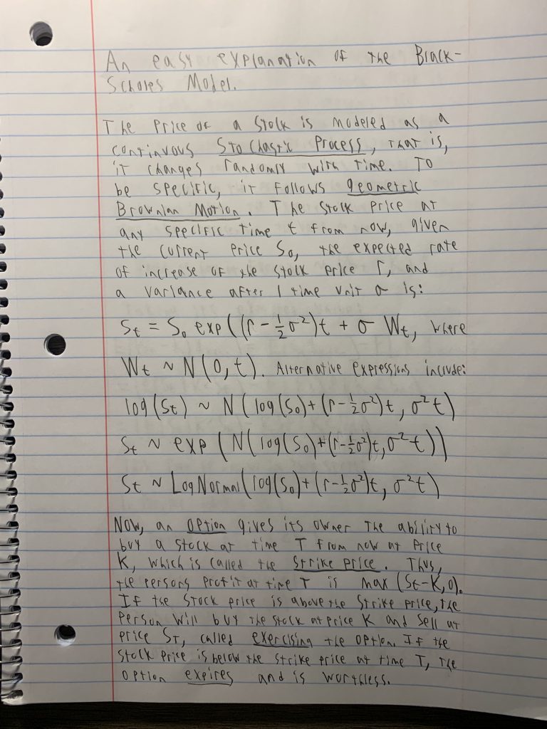
Recently I’ve been reading about Happy Harry et al’s “Adventures in Stochastic Processes” by Sidney I. Resnick in order to prepare for the course in Survival Analysis I’ll be taking next semester with professor David Oakes, and since I’ve been haphazardly skipping around the book, I went to the chapter on Brownian Motion earlier today and I was expecting to find a lot of material that could easily relate to the Stock Market, as I’ve heard many times that the movement of a stock is typically modeled with Brownian motion. However I wasn’t sure I could see the connection right away from the text, and so I went to Chat-GPT, which told me that the stock market is an example of Geometric Brownian Motion, a close cousin of Standard Brownian Motion. I also finally figured out how to install a plugin to let my type latex (the plugin is called QuickLatex), so I’m going to demonstrate that with the following definition of Standard Brownian Motion:

(1) $\begin{equation*} $W_{t+h} - W_t \sim N(0, h)$ \end{equation*}$

Basically, what this means is that where you are, W (W stands for Weiner, as in the Weiner process, not where), changes with time, and your location at time t is $W_t$ , and the change between where you are at time t and where you are at time t+h follows a normal distribution with greater variance the greater time h between right now (t) and time h. Clearly this Stochastic Process has the Martingale Property (at any time t the expected value of where you are at h is where you are at t) and is a Markov process (it doesn’t remember where you were before time t). Stock prices are modeled as following Geometric Brownian Motion, which is this ( $S_t$ is the price at $t$ which is now a time t in the future from now, $S_0$ is the price now):

(2) $\begin{equation*}$S_{t} = S_{0}e^{((r-\frac{1}{2} \sigma^2)t + \sigma W_t)}$\end{equation*}$

Where r is the rate of return and W is the Weiner process. Since $W_t$ is just a normal random variable for a fixed t, let’s say T, this is also equivalent to $S_T$ being a lognormal random variable, that is:

(3) $\begin{equation*}$\log(S_T) = \log(S_0) + \left( r - \frac{\sigma^2}{2} \right) t + \sigma W_T \sim N(\log(S_0) + \left( r - \frac{\sigma^2}{2} \right) T, T \sigma^2)$\end{equation*}$

(4) $\begin{equation*}$S_T \sim LogNormal(\log(S_0) + \left( r - \frac{\sigma^2}{2} \right) T, T \sigma^2)$\end{equation*}$

Now chat-GPT then threw me for a loop by telling me that the Black-Scholes equation based on this model gives you the following formula for determining the price $C(S_0, t)$ of a call option with risk-free rate of return r, current price $S_0$ , strike price K, variance $\sigma^2$ (which can be thought of for the business minded as controlling the volatility), and time until maturity T, as (I wrote d_1 in terms of d_2 and sigma, but writing it the other way is what Chat-GPT did and what is more common, but I prefer this way and you’ll see why later):

(5) $\begin{equation*}$C(S_0, T) = S_0 \Phi(d_1) - K e^{-rT} \Phi(d_2)$\end{equation*}$

Where

(6) $\begin{equation*}$d_2 = \frac{\log\left(\frac{S_0}{K}\right) + \left( r - \frac{\sigma^2}{2} \right)T}{\sigma \sqrt{T}}$\end{equation*}$

(7) $\begin{equation*}$d_1 = d_2 + \sigma \sqrt{T}$\end{equation*}$

$\Phi$ of course represents the standard normal cumulative density function. Further prompting of Chat-GPT was unhelpful, but luckily I have a teeny bit (a lot of bit) of background in statistics, and as a result of my inherent curiosity I got sucked in and had to spend the day figuring out what was going on here. Luckily I was eventually able to work out where this was coming from (with the help of another blog that gave me the key component: the expected value of the truncated log-normal distribution). Now for the fun part; I’m going to derive the above Black-Scholes price formula above using only the previously given information about $S_t$ as a lognormal random variable. No need to bring out the differential equations.

First, for the non Wall Street minded, let’s explain what a Call Option (a Call) is. A Call gives its owner the ability to buy a stock at time T from now (we don’t consider the case where you can sell before time T, we’re working with what are called European options) at a price K, which is called the strike price. Obviously if the price of the stock is below the strike price at time T, the option is worthless because it’d be better to just buy the stock at the market price than to use your option. However, if the stock price is above the strike price at time T, the option is worth $S_T - K$ to you, you only have to pay $K$ for the stock, but the stock is worth $S_T$ . Actually using the option to buy the stock (which is then usually sold again immediately to make profit $S_T - K$ ) is called exercising the option. If the stock price is below the price of the option at time T, the option is said to have expired worthless.

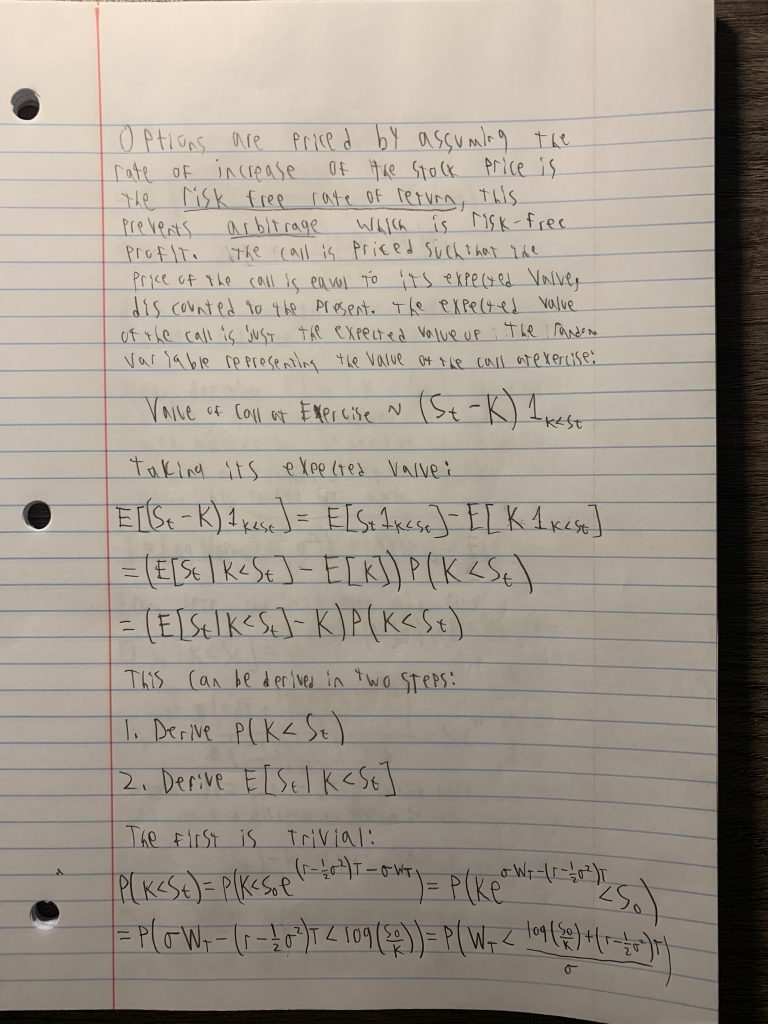
Options are priced by assuming the rate of increase of the stock price is the risk free rate of return, which prevents arbitrage which is risk free profit. The call is priced such that the price of the call is equal to its expected value under the aforementioned model of the price of a stock given by Geometric Brownian Motion, discounted to present (which means that the amount of money you are expected to make at time T has to be put into today’s terms using the risk free interest rate, which is done by just multiplying by $e^{-rT}$ ). Now it’s not very difficult to realize that amount of money you make at exercise is the following random variable:

$(S_T - K)\textbf{1}_{K < S_T}$

The option is worth $S_T - K$ if the stock price is over K at the time of exercise, and zero otherwise. Thus the expected value the option at the time of exercise is:

$\mathbb{E}[(S_T - K)\textbf{1}_{K < S_T}] = \mathbb{E}[S_T\textbf{1}_{K < S_T}] - \mathbb{E}[K\textbf{1}_{K < S_T}] = \mathbb{E}[S_T | K < S_t]\mathbb{P}(K<S_T) - K\mathbb{P}(K<S_T)$

$= (\mathbb{E}[S_t | K < S_T] - K)\mathbb{P}(K<S_T)$

Now we can derive the Call pricing formula in three steps:

Derive $\mathbb{P}(K<S_T)$
Derive $\mathbb{E}[S_t | K < S_T]$
Plug in and discount to present

The first step isn’t too difficult, just sub in (2) and do some algebra and the result comes right out:

$\mathbb{P}(K < S_T) = P(K < S_0e^{(r-\frac{1}{2}\sigma^2)T - \sigma W_T}) = \mathbb{P}(Ke^{\sigma W_T - (r - \frac{1}{2} \sigma^2)T} < S_0) = \mathbb{P}(\sigma W_T - (r-\frac{1}{2}\sigma^2)T < \log(S_0/K))$

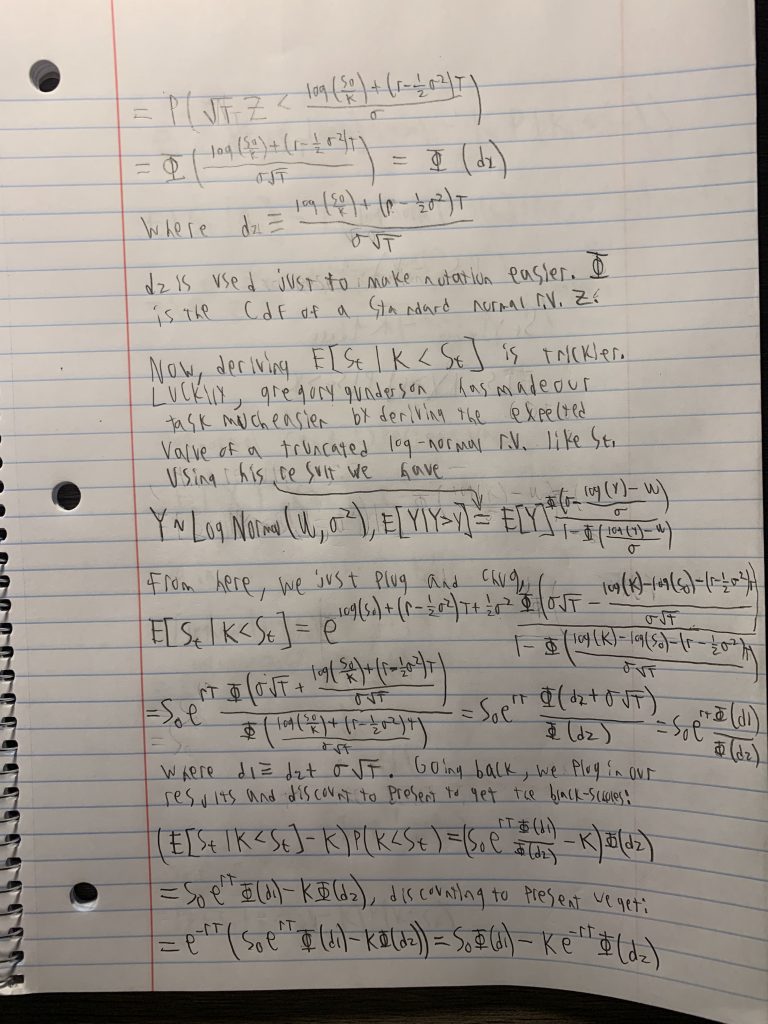
$= P(W_T < \frac{log(S_0/K) + (r-\frac{1}{2}\sigma^2)T}{\sigma}) = P(Z < \frac{\log(S_0/K) + (r-\frac{1}{2}\sigma^2)T}{\sigma\sqrt{T}}) = \Phi(\frac{\log(\frac{S_0}{K}) + (r-\frac{1}{2}\sigma^2)T}{\sigma\sqrt{T}}) = \Phi(d2)$

Remember when I said it was easier to write d2 out explicitly and write d1 as d2 + $\sigma\sqrt{T}$ ? Because we wrote it that way, we can see easily that the above term reduces to $\Phi(d2)$ .

Deriving $\mathbb{E}[S_T | K < S_T]$ is trickier. Luckily, I had some help from another blog I found online! Greg Gunderson demonstrated with a small but clever proof of the expected value of a truncated lognormal random variable. The link can be found here.

From Greg we learn the following fact: If Y is a Lognormal random variable with parameters $\mu$ and $\sigma^2$ (the mean and variance of the normal that is in the exponent), and we truncate the probability distribution of Y such that Y has zero probability for Y < y, and the rest of the probability distribution is scaled accordingly, the expected value of this new random variable $Y | y < Y$ is given by

$\mathbb{E}[Y | y < Y] = E[Y] \frac{\Phi(\sigma - \frac{log(y) - \mu}{\sigma})}{1-\Phi(\frac{log(y) - \mu}{\sigma})}$

It turns out, this little fact is all we need! This and the expected value of a LogNormal random variable, which is well known to be $e^{\mu + \frac{1}{2}\sigma^2}$

Recall from (4) that $S_t$ is LogNormally distributed, so plugging in $\log(S_0) + \left( r - \frac{\sigma^2}{2} \right) T$ for $\mu$ and $T \sigma^2$ for $\sigma^2$ gives:

$\mathbb{E}[S_T | K < S_T] = E[S_T] \frac{\Phi(\sigma\sqrt{T} - \frac{\log(K) - \log(S_0) - \left( r - \frac{\sigma^2}{2}\right)}{\sigma\sqrt{T}})}{1-\Phi(\frac{log(K) - \log(S_0) - \left( r - \frac{\sigma^2}{2}\right)}{\sigma\sqrt{T}})} = e^{\log(S_0) + (r-\frac{\sigma^2}{2})T + \frac{\sigma^2}{2}T} \frac{\Phi(\sigma\sqrt{T} + \frac{\log(S_0/K) + \left( r - \frac{\sigma^2}{2}\right)}{\sigma\sqrt{T}})}{\Phi(\frac{\log(S_0/K) + \left( r - \frac{\sigma^2}{2}\right)}{\sigma\sqrt{T}})}$

$= S_0 e^{rT} \frac{\Phi(d2 + \sigma\sqrt{T})}{\Phi(d2)} = S_0 e^{rT} \frac{\Phi(d1)}{\Phi(d2)}$

The last steps are trivial:

$(\mathbb{E}[S_T | K < S_T] - K)\mathbb{P}(K<S_T) = (S_0 e^{rT} \frac{\Phi(d1)}{\Phi(d2)} - K)\Phi(d2) = S_0 e^{rT}\Phi(d1)} - K\Phi(d2)$

This is the expected value of the call at exercise. To get the price of the call, we just take this and discount it to present:

$(S_0 e^{rT}\Phi(d1)} - K\Phi(d2))e^{-rT} = S_0 \Phi(d1) - Ke^{-rT}\Phi(d2)$

Which is the Black-Scholes formula for the price of a European call option.

Overall, I’ve had a fun Saturday with this and I look forward to learning more about Stochastic processes. Some of my notes (redundant with the above):

Leave a Comment Cancel Reply