Optimizing a Dynamic Treatment Regime, David Skrill awarded his PhD, and my Self-Study plan

3:44 AM, November 24, 2024

Long blog post today. As I mentioned in the previous blog post, I’ve come up with a plan for self-study, and there are a couple of other developments in my plans for the program that I’ll share at the end of this blog post. Also, my friend David Skrill was just awarded his PhD. And I’ll get to all that, but first I’d like to as promised talk a bit about Dynamic Treatment Regimes (DTRs), which I did a presentation on for my Causal Inference class, which can also be found in the previous blog post. The information comes from the paper by Philip J Schulte and Butch Tsiatis, Q and A learning for estimating optimal dynamic treatment regimes.

The motivation for DTRs is that in clinical practice it is rare that a patient actually be given only a single treatment and that drug be used throughout the treatment plan, instead a patient is given a treatment and based on how they respond to the treatment (ie how their covariates change) the physician might change their treatment. A dynamic treatment regime is a sequence of rules, each rule takes the patients covariates and their past treatment history as an input and returns a treatment as an output. When forming a DTR, we typically think of the treatment as occurring in ’rounds’, the first round is the patients initial assignment to treatment, and each subsequent round is an opportunity for the physician to switch their treatment or keep them on the same treatment. In math language, the rounds are often notated:

$k \in 1, 2, …, K$

1 being the first round and K being the last. The set of possible treatments at decision point k is $\mathbb{A}_k$ , where a single possible action at round k is written $a_k \in \mathbb{A}_k$ . At decision point k, the patient’s covariates (and covariate history) which is their ‘state’ and treatment history or ‘action’ history, we can call the ‘state action history’ and write as $\bar{s}_k, \bar{a}_{k-1}$ , where the overline just indicates all of the things leading up to k (or k-1). The set of possible states at $k$ is $S_k$ . Sometimes, certain actions are not permitted if a patient has a particular history, eg if they had an allergic reaction to a drug in the past, so the allowed actions at point $k$ is a function of the state-action history, and in this case we write the allowed actions at time point $k$ as $\Psi(\bar{s}_k, \bar{a}_{k-1})$ . The final outcome of interest after all treatments (eg remission status) is notated $Y$ .

The dynamic treatment regime is a set of functions $d = (d_1(s_1), d_2(s_2, a_1), d_3(s_3, \bar{a}2), … d_K(s_K, \bar{a}{K-1}))$ that determine how a patient should be treated given any possible current covariates and past treatment history. Each patient in the set of patients (notated $\omega \in \Omega$ ) has potential outcomes that reflects how their covariates would have changed and how their final outcome would have changed if they had been given any particular set of treatments, written as $S^*_2(d_1), …, S^*_k(\bar{d}_{k-1}),…,S^*_K(\bar{d}_{K-1}), Y^*(\bar{d}_K))$ .

The optimal regime is the one that maximizes the expected value of a patients potential outcome $Y^*(\bar{d}_K)$ , so we write $\mathbb{E}[Y^(d) | S_1 = s_1] \leq \mathbb{E}[Y^(d^{\textrm{opt}}) | S_1 = s_1] \textrm{ }\forall d \in \mathbb{D} \textrm{ and } \forall s_1 \in \mathbb{S}_1$ , where $D$ is the set of all possible dynamic treatment regimes. The trouble of course, as in all causal inference, comes from the fact that for each patient we only observe the outcome that actually happens for them, and can’t observe all of their potential outcomes. This is also why we have to assume the outcomes and covariates observed are the potential outcomes and covariates under the treatments actually administered. We also make the Stable Unit Treatment Value Assumption (the patient’s covariates and outcomes are unaffected by how other patients are treated). If the data are from a special type of clinical trial designed to infer a DTR called a SMART (Sequential Multiple Assignment Randomized Trial), then we have random assignment. If not, we have to assume no unmeasured confounders.

Two methods for estimating the optimal dynamic treatment regime are Q-learning and A-learning. Both learning methods for the dynamic treatment regime are done by backwards induction, so that your model for round k is only conditional on the past, not the future. If you threw your action at all time points into, say, one model linear model for outcome, then the coefficients of the decisions at different time points would be interpreted as being conditional on future outcomes. Recall that, in a linear model, the coefficient for $\beta_k$ is interpreted as the expected change in y for a 1 unit change in $x_k$ holding all else equal. But in this case we don’t want to hold the future equal, so we have to do backwards induction. Essentially, what you do is fit a model at the last round, which takes the action taken at the last time point, the actions taken at all previous time points, and the states at all previous time points, as predictors, and use that model to predict outcome. Then, once you have that model, determine for each patient, based on their covariates other than the current treatment and the model, what their predicted outcome would have been under both treatments, and take the maximum of the predicted outcomes under treatments available at that time point (this maximum is called the Value), and use that as the outcome for a model that does the same thing at round k-1, and repeat this process until you get all the way back to round 1. Then all of the models you’ve trained give you the estimated optimal dynamic treatment regime.

Q- learning and A-learning are two different ways of performing this process. Q-learning models the quality of each treatment (the model for outcome) directly, while A-learning which is used when there are only two treatment options models the outcome as the sum of a contrast function (which gives the difference between the two treatments) and a function that only depends on the covariates and past treatment history. The estimating equation for the Q-functions (eg the outcome or the backwards inducted ‘outcome’ created by the models for future rounds) is

$\sum_{i=1}^n \frac{\partial Q_k (\bar{S}_{ki}, \bar{A}_{ki}; \xi_k)}{\partial \xi_k} \Sigma_k^{-1} (\bar{S}_{k, i}, \bar{A}_{k,i}) \times { \hat{V}_{(k+1),i} - Q_k(\bar{S}_{k, i}, \bar{A}_{k,i}; \xi_k) } = 0$

Where the $\Sigma$ is the variance structure. All you really need to know for the purpose of reading the rest of the blog post is that this more or less just lets us estimate the parameters of the assumed models $Q_k$ at each of the $K$ rounds, each of which uses $V_{k+1}$ as the outcome variable, except for the last round which uses $Y$ as the outcome variable.

The value V is defined as

$V^{(1)}_{K-1} \left( \bar{s}_{K-1}, \bar{a}_{K-2} \right) = \max{a_{K-1} \in \Psi_{K-1} (\bar{s}_{K-1}, \bar{a}_{K-2})} E [ V^{(1)}_K (\bar{a}_{K-2}, a_{K-1}) \mid \bar{S}^{*}_{K-1}(\bar{a}_{K-2}) = \bar{s}_{K-1} ]$

, the Q function evaluated at the optimal treatment for the patient at that time point.

This is probably confusing, so let me illustrate with a simple example. Let’s say you have the data of 64 patients, and those patients can be assigned to treatments A or B at each round, and there are two rounds. The goal is to reduce blood pressure, where blood pressure reduction is the outcome. 16 patients go A then A, 16 go A then B, 16 go B then A, 16 go B then B. There is a covariate, which is whether the person has heart disease, and in each group half of the patients have heart disease. The following average outcomes (reductions in blood pressure after both treatments) are observed:

Heart Disease: AA = 4, AB = 0, BA = 0, BB = 8 Healthy: AA = 4, AB = 0, BA = 0, BB = 0

Obviously, healthy patients should receive AA and heart disease patients should receive BB. What we are doing is this: pose a model at round 2 for outcome:

$Y = \beta_0 + \beta_A x_A + \beta_H x_H + \beta_{prev A} x_{prev A} + \beta_{H, prevA} x_H x_{prev A} + \beta_{prev A, H, A} x_{prev A} x_H x_A$

When we fit this model, the result will be a model that predicts high outcomes for people who were previously treated with A who received A again, and even higher outcomes for people who were previously treated with B and received B again and who have heart disease. We then take the prediction of this model for each patient under a round 2 treatment A or treatment B, and take the maximum of those two predictions and recurse it backwards. What this does is predicts the same ‘value’ for people who were treated with A in round 2 and B in round 2, so that the model for round 1 doesn’t depend on what you were ACTUALLY assigned in round 2, it depends only on what the best thing you COULD have been assigned in round 2. This prevents you from making the wrong decision at round 1 because of what was assigned in round 2. For example, let’s say almost all of the people with heart disease treated with B in round 1 were then switched to A, it might look like B is just a worse treatment, but the problem was that the treatment in round 1 was usually not followed up with the best treatment in round 2 for people treated with B in round 1, which is to treat with B again. By taking only the predicted outcome under the best treatment in round 2, you remove this problem from the round 1 model. Using this predicted outcome under the best treatment in round 2, V, you then fit the round 1 model, let’s pose it as:

$V = \beta_0 + \beta_A x_A + \beta_H x_H + \beta_{H, A} x_H x_A$

Then you fit this model, and you’re done. And you can apply this same general method to more complicated situations. The Q-function estimating equations I gave above were for Q-learning, A-learning estimating equations look like this:

$\sum_{i=1}^{n} \frac{\partial}{\partial \psi_k} C({\bar{S}k,\bar{A}{k-1}; \psi_k})\left{ A_{k i} - \pi_k \left( \overline{S}{k i}, \overline{A}{(k-1) i}; \phi_k \right) \right}$

$\times { \tilde{V}{(k+1) i} - A{k i} C_k \left( \overline{S}{k i}, \overline{A}{(k-1) i}; \psi_k \right)- h_k ( \bar{S}{k i}, \bar{A}{(k-1) i}; \beta_k ) } = 0$

$\sum_{i=1}^{n} \frac{\partial h_k \left( \overline{S}{k}, \overline{A}{(k-1)}; \beta_k \right)}{\partial \beta_k} { \tilde{V}{(k+1) i} - A{k i} C_k ( \overline{S}{k i}, \overline{A}{(k-1) i}; \psi_k ) -$

$h_k ( \overline{S}{k i}, \overline{A}{(k-1) i}; \beta_k ) } = 0$

Which is essentially just saying that you model the part of the Q-function that is the difference between treatment (C for contrast) and the part that depends only on the past (h for history) as separate functions, and you propose a propensity model $\pi$ . Entire books have been written on the subject of adjustment for propensity of treatment which is something done in many other contexts than this one, so maybe I’ll make another blog post just on that subject. Whenever you do a propensity score matching or an IPW or an AIPW, you’re adjusting for the propensity of treatment, which is a way of removing the effect of the fact that people with some covariates might be more likely to receive treatment than those with different covariates when you don’t have randomization. The main tradeoff between Q and A learning is that A learning tends to be more robust to model misspecification and Q learning tends to be more efficient. Anyway, as I sit here blogging my girlfriend has gone to bed and about 16 cops have pulled up outside and are knocking on the doors of people living nearby, but this is Rochester so it’s not a shocking thing to happen, but somehow it tells me I should probably wrap this up. There’s a lot of complexity here for someone not familiar with the subject, I spent significantly more time reading about and trying to understand these methods than I did actually making the presentation itself (which was also time consuming in and of itself), but it counted for my midterm grade in the course so I wanted to make it good. I mostly just really wanted to understand it for its own sake though. I think this potentially hasn’t been the best blog post, as looking back through it I don’t think I’d really understand what was going on from the blog post if I wasn’t coming at it with prior knowledge of DTR. I think it just needs a more full treatment than I’ve given it here. Look through the presentation in the previous blog post if you’re really curious, I think the presentation does a better job than I’ve done in the blog post. Nevertheless, I enjoyed writing this.

Wrapping back, David Skrill, who is another PhD student several years ahead of me in the Statistic PhD program and who I’ve gotten to know through Sam Norman-Haignere’s lab, was awarded his PhD on Friday! He did a wonderful job in his clear and articulate dissertation talk about the component-encoding models he developed to combine the interpretability of component models with the predictive power of encoding models for modeling neural responses to natural stimuli in the brain, and behind closed doors I imagine he did just as well in his defense to the committee. To celebrate the whole lab went to Lasertron Henrietta and played Laser Tag and Arcade games. I managed to score a good amount of points in the laser tag because I figured out how to change to “spy mode” which let me look temporarily like I was on the opposing team, so I could run into their base and score a zillion points on it while they weren’t paying attention. Eventually people caught on and zapped me though. More importantly, we all had a blast there. Since significant others were invited I was able to bring my girlfriend as well, as you can see in the nice photo below. Credit to the amazing Li Zehua (who showed us all his very cool pair of Ray-Ban Meta glasses, Meta really is broadening its horizons as a tech company of late).

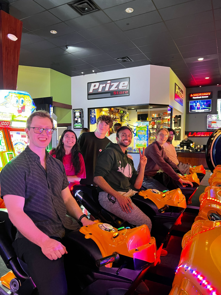
From left to right: Freshly minted Dr. David Skrill who earned his PhD on Friday, my girlfriend Olivia, Me, Abhi, Joseph, Akhil, and in the way back behind the computer you can see Josh, the Lasertron employee who gave us arcade tokens that we *technically* weren’t supposed to have.

As for my self-study plan, I’ve figured out a loose idea, but I have not hammered it down exactly yet, and I also still have yet to figure out exactly what I’m doing next semester yet with one of my course slots that I had planned to use for genomic data analysis, but genomic was scheduled at the same time as one of my other classes, but then I got really excited about using that free spot to do a reading course with a professor about Dynamic Treatment Regimes, but that professor was not going to be able to do it for reasons that will be explained eventually, but can’t be posted online at the moment. I then asked a different professor who does similar work about doing a reading course on the subject, and he also was not going to be able to do it next semester for an entirely different reason that will also be explained at a later date but I also can’t post online now. Both said they would have been enthusiastic about giving me a reading course on the topic had circumstances worked better, and both had very good reasons. So I’m unsure exactly what my plan is.

I’m also trying to TA the Statistical Inference II: Large Sample Theory course being taught next semester, which I took last Spring. I mostly want to TA it because it will force me to learn and really understand the material of the course, which I want to do for its own sake but also so that I can nail it on the Advanced Exam next August. Which brings me to the loose idea for a study plan, starting with the stuff I want to do to prepare for Survival Analysis next semester. First, I think I’m going to read the chapter of the (upper level undergraduate) textbook Intro to Stochastic Processes in R that has to do with Poisson Processes (Chapter 6), and then with that context I will read (and probably still not understand a lot of) chapter 3 and 4 of Adventures in Stochastic Processes which is the much more challenging Resnick book I mentioned in the previous post about the LogNormal distribution and its connection to Option pricing. I’m going to make a post about each of these three chapters, preferably one week after another, so I’ll try to post about the poisson process by the first week of December, the Stochastic process book chapter 3 the week after that, and chapter 4 the following week. It also works out nicely that chapters three and four of the Resnick book are right after chapter 2, which I’ve read some of (learned what a markov chain is and a transition matrix) but will skip the bulk of (it’s quite a long chapter) and then hopefully come back to eventually. Maybe I’ll do one read through of the rest of chapter 2 without stopping to really fully conceptualize everything I’m reading, which is the hard part of reading a textbook. Reading the words and mathematical statements is easy enough, the “Why is that true? Why does that make sense? What’s the intuition here?” self questioning and self justification of what you’re reading which brings the real understanding of the material is the part that takes a long time. Then, once I finish up learning about Poisson processes to the point where I feel reasonably prepared for Survival, it’ll be about mid-December, and I’ll dive into Van Der Vaart Asymptotic Statistics, and probably not understand a lot of it, but I’ll also be going though old course notes Large Sample Theory, and I have some other notes I found online to supplement what I already have. I’ll work though all that during my holiday break and then continuing into January and the next semester while I (hopefully) TA the course, and I’ll make regular blog posts about different things in Asymptotic statistics I’m learning. During the spring semester, I’ll also hopefully have found a professor to learn something interesting with, and I’ll also have that to potentially post about as well. I could also maybe just do a reading course with Sally and use that to really focus on the work I’m doing for the longitudinal analysis of postnatal methylmercury exposure for the children in the Seychelles child development study. I also totally finally found a source that explained REML and why its different than ML for longitudinal LMEM models in a way that actually made sense to me, and that gave me a deep sense of relief. That could also be another blog post, but just quickly what it has to do with is that you multiply y by some vectors a that have the property that aX = 0, so that ay = aX beta + aZb+ a epsilon removes the aXbeta, where X is the fixed effects stuff and Z is the random effects stuff and then you do some algebra and you get the ML of the variance structure of b for this (because all random effects are assumed to have a normal distribution centered at 0, so you use ML to find the variance of the random effect), and then you put that variance structure in and estimate the fixed effects, and this result is unbiased for the variance, whereas ML without this adjustment over-estimates the variance terms because it doesn’t account for the fact that some of the same data is used to estimate the fixed effects. At some point a blog post about REML might be good as it took me a long time to find a source that actually explained it well.

The last few weeks I’ve been very busy with coursework (and by ‘coursework’ I mostly mean the steep learning curve and long computation times of High Dimensional data analysis) and I haven’t had a lot of time to devote to the cluster ensembling research I’m doing with Luke, which luckily has worked out fine since he’s also been super busy applying for and interviewing for jobs in addition to his work at the TH Chan school of Public Health as a Postdoc, as he’s trying to get a position as a professor for when he finishes the Postdoc. Hopefully, fingers crossed, he manages to snag the open position they’re trying to fill within the department here at the University of Rochester.

Another thing I’ll say is that lately I’ve felt more an more assured of my own competence and that I actually do belong in this PhD program, and that I am understanding things and have built up a good intuition for statistics, and I’ve also gotten a lot closer with other members of the co-hort and enjoy talking to them about stats, classes, and a litany of other things. I really am incredibly grateful to be where I am, getting to spend so much of my time just learning about interesting things and getting to use my brain on a daily basis. For those who love thinking as much as I do, I can’t imagine anything that’s as cool to do as your work as a young person as being a grad student in a PhD program. I’ve also learned to appreciate the fact that unless you’re good Will Hunting you just won’t understand everything you’re trying to learn as quickly as grad school throws it at you, especially not right away, and that that’s perfectly normal. The other thing that’s become more apparent to me lately, as I think I mentioned in the last blog post, is how much more you can get done maintaining singular focus on whatever task is immediately in front of you and drowning out the brain noise that’s trying to distract you by getting you to think about all the other things that you have on your plate than you can get done trying to multitask and do everything at once. Focus. That’s what it’s about.

With luck I’ll have my next blog post up about a week from now, although I’ll be pretty busy over the Thanksgiving break, since I’m doing Thanksgiving with my family and extended family at Grandpa’s cottage on Conesus lake, and then I’m doing a Friendsgiving on Friday, where me and a bunch of friends who graduated from the U of R last year (because they were seniors at the U of R when I was in the first year of my PhD) are all going to an Airbnb in Earlton (basically into the woods of central NY) and staying there Friday and Saturday and coming back Sunday. So it might be two weeks from now until I do another blog post. I’ve been really enjoying blogging and I hope that I continue to scrape out time to do it. Until next week!

Leave a Comment Cancel Reply