6:02 PM, October 23rd, 2024
Today I had the opportunity to present on the topic of measurement error for my Statistical Seminar course. I felt that outside of a lot of “umms” and “ahhs” the presentation went well, based on the questions I got during the questions portion at the end people seemed to understand the material, and my advisor for the paper Sally Thurston said she thought the presentation was good. I personally think that I used some ambiguous language at certain points, i.e. “this Bayesian thing” or using the word “significant” when I wasn’t actually referring to statistical significance, and I definitely have room to improve my presentation skills. Also, my girlfriend and one of her friend’s from the Simon Business school were in attendance, which I enjoyed, and they said they understood more than they expected to, which means I did a reasonably good job explaining things if even non-statisticians had an idea of what I was talking about. It’s rather surprising the number of presentations that I see, even in the colloquium, that are mostly incomprehensible to those who have statistical background but not in the area of research of the presenter. Although maybe it’s more incomprehensible to me than everyone else, I don’t want to blame presenters entirely when the problem could just be my own ignorance. I really just think it would be nice if presenters assumed the audience had significantly less knowledge and/or ability to understand new concepts quickly than they typically do.
The topic of measurement error itself was interesting to me, and the authors of the paper published the code in a repository for some of their analysis of the NHANES III data that they used (comparing it to Regression Calibration) and I was able to run it on my own device which I found helpful. I think that authors ought to make code like this public more often. For example, they ran a lot of simulations comparing regression calibration to the bayesian method, but none of that code was in the repo. I also think that they could have structured the paper a little bit differently. The paper was largely making the argument that Bayesian corrections for measurement errors and well known and developed but are not used frequently enough by non-bayesian statisticians and epidemiologists. And they say that the simulation results are similar for the Bayesian and Frequentist methods, but in the actual simulation results they give the RC is centered at the truth and has much smaller CI’s especially in the simpler cases or the cases where Beta_X is small. The simulations however revealed that sometimes the RC method has a tendency to underestimate the true parameter when Beta_X is large, ie larger than 2 when all variables are centered and scaled. I think they ought to have put more emphasis on the fact that the main benefit of the use of Bayesian methods in addressing measurement error is that you can fit models that are much more complex than is possible for RC, and that there is a practical ease to using Bayesian methods in complex settings in that you can just set up all of the complex relationships missingness and measurements with error and the MCMC will (presuming it converges) give valid inferences and credible intervals, and as n goes to infinity the bayes estimator is normal, efficient, etcetera. They also should’ve put more emphasis on the fact that specifically for the Cox regression the Bayes estimator performs as well or better than RC, although I think that they didn’t want to emphasize this largely because on the NHANES III data they were unable to use Cox regression because of how long it takes to fit. Maybe it’d be sort of like saying “oh here’s this great method that works really well for this type of data, but it takes an eternity to fit.” Alas, I digress.
Below you can find the presentation, as well as the code I wrote for the simple simulations I talked about in the presentation. The link to Keogh’s repository can be found here.
I’m partially upset that in my presentation I didn’t include a joke about how ‘convergence’ to Bayesians usually means convergence of the MCMC sampler (meaning the sampler no longer depends on the initial values), and not ‘covergence’ in the frequentist sense (i.e. convergence of the estimator to the parameter it estimates).
R Code:
Used to generate visualizations in earlier parts of presentation:
library(“ggplot2”)
set.seed(224)
n <- 500
beta_0 <- 1
beta_1 <- 3
sigma_x <- 1
sigma_w <- 1
sigma_epsilon <- sqrt(2)
data.x <- rnorm(n, mean = 0, sd = sigma_x)
data.w <- data.x + rnorm(n, mean = 0, sd = sigma_w)
epsilon <- rnorm(n, mean = 0, sd = sigma_epsilon)
data.y <- beta_0 + beta_1 * data.x + epsilon
gold_index <- sample(1:500, 50)
cal_gold <- lm(data.x[gold_index] ~ 0 + data.w[gold_index])
calibrate_gold <- function(w){
w*as.numeric(cal_gold$coefficients)
}
rep_index <- sample(1:500, 100)
data.w.rep <- data.x[rep_index] + rnorm(100, mean = 0, sd = 1)
cal_repeat <- lm(data.w.rep ~ 0 + data.w[rep_index])
calibrate_repeat <- function(w){
w*as.numeric(cal_repeat$coefficients)
}
data <- data.frame(x = data.x, y = data.y, w = data.w)
Load the ggplot2 library
library(ggplot2)
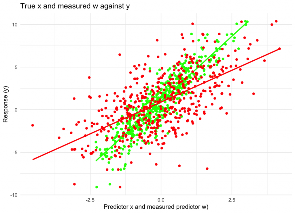
ggplot(data, aes(x = x, y = y)) +
geom_point(color = “green”) +
geom_smooth(method = “lm”, se = FALSE, color = “green”) +
geom_point(aes(x = w, y = y), color = “red”) +
geom_smooth(aes(x = w, y = y), method = “lm”, se = FALSE, color = “red”) +
labs(x = “Predictor x and measured predictor w)”, y = “Response (y)”,
title = “True x and measured w against y”) +
theme_minimal()
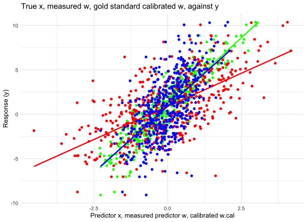
ggplot(data, aes(x = x, y = y)) +
geom_point(color = “green”) +
geom_smooth(method = “lm”, se = FALSE, color = “green”) +
geom_point(aes(x = w, y = y), color = “red”) +
geom_smooth(aes(x = w, y = y), method = “lm”, se = FALSE, color = “red”) +
geom_point(aes(x = calibrate_gold(w), y = y), color = “blue”) +
geom_smooth(aes(x = calibrate_gold(w), y = y), method = “lm”, se = FALSE, color = “blue”) +
labs(x = “Predictor x, measured predictor w, calibrated w.cal”, y = “Response (y)”,
title = “True x, measured w, gold standard calibrated w, against y”) +
theme_minimal()
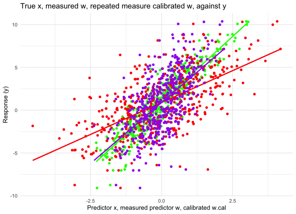
ggplot(data, aes(x = x, y = y)) +
geom_point(color = “green”) +
geom_smooth(method = “lm”, se = FALSE, color = “green”) +
geom_point(aes(x = w, y = y), color = “red”) +
geom_smooth(aes(x = w, y = y), method = “lm”, se = FALSE, color = “red”) +
geom_point(aes(x = calibrate_repeat(w), y = y), color = “purple”) +
geom_smooth(aes(x = calibrate_repeat(w), y = y), method = “lm”, se = FALSE, color = “purple”) +
labs(x = “Predictor x, measured predictor w, calibrated w.cal”, y = “Response (y)”,
title = “True x, measured w, repeated measure calibrated w, against y”) +
theme_minimal()
set.seed(224) # For reproducibility
Parameters
n <- 10000
beta_0 <- 1
beta_1 <- 3
sigma_x <- 1
sigma_w <- 1
sigma_epsilon <- sqrt(2)
1. Generate true x values
X <- rnorm(n, mean = 0, sd = sigma_x)
2. Generate w values with measurement error
W <- X + rnorm(n, mean = 0, sd = sigma_w)
3. Select x values to create duplicate w values
dup_indices <- sample(1:n, 500)
dup_W <- X[dup_indices] + rnorm(500, mean = 0, sd = sigma_w)
4. Generate y values from the true x
epsilon <- rnorm(n, mean = 0, sd = sigma_epsilon)
Y <- beta_0 + beta_1 * X + epsilon
5. Print w and y data, and duplicates
data <- data.frame(
Y = Y,
W = W
)
head(data)
summary(lm(Y ~ W))
6. Run Regression Calibration Approach
cal <- lm(dup_W ~ W[dup_indices])
summary(cal)
calibrate <- function(w){
w*as.numeric(cal$coefficients)
}
summary(lm(Y~calibrate(W)))
7. Estimate sigma_w
sigma_w_squared_estimate = ((1/(500-1))*sum(((dup_W – W[dup_indices]) – mean(dup_W – W[dup_indices]))^2))/2
sigma_w_squared_estimate
In theory sigma_w should have diffuse prior, but I had trouble implementing it in rjags,
So I just used the point estimate of sigma_w_squared based on the sample standard deviation,
which root-n converges to the true value of sigma_w_squared as the sample size increases
8. Implement the Bayesian error correction in Jags
library(rjags)
Define the JAGS model
model_string <- “
model {
# Outcome model
for (i in 1:N) {
Y[i] ~ dnorm(beta0 + beta1 * X[i], tau_epsilon)
}
# Measurement model
for (i in 1:N) {
W[i] ~ dnorm(X[i], tau_u)
}
# Latent variable model
for (i in 1:N) {
X[i] ~ dnorm(0, tau_x)
}
# Priors
beta0 ~ dnorm(0, 1.0E-6)
beta1 ~ dnorm(0, 1.0E-6)
tau_epsilon ~ dgamma(0.5, 2)
tau_x ~ dgamma(0.5, 2)
# Known precision for the measurement error
tau_u <- 1 / sigma_u_squared
}”
Data preparation
data_list <- list(
N = nrow(data),
Y = data$Y,
W = data$W,
sigma_u_squared = sigma_w_squared_estimate # Known measurement error variance
)
Initial values
init_list <- list(
beta0 = 0,
beta1 = 0,
tau_epsilon = 1,
tau_x = 1
)
Parameters to monitor
parameters <- c(“beta0”, “beta1”, “tau_epsilon”, “tau_x”)
Run the JAGS model
jags_model <- jags.model(
textConnection(model_string),
data = data_list,
inits = init_list,
n.chains = 3,
n.adapt = 500
)
Burn-in
update(jags_model, n.iter = 1000)
Sampling
samples <- coda.samples(
jags_model,
variable.names = parameters,
n.iter = 5000
)
Summarize results
summary(samples)